3  其他分类算法 (机器学习)

你正在阅读的是正在进行中的关于 《根据测试集中的论文摘要自动提取关键词》 的研究报告本章节处于打磨阶段: 其内容基本完备, 但是仍在打磨中。

3.1 Setup

import numpy as np
import pandas as pd
import os
from sklearn.feature_extraction.text import CountVectorizer
from sklearn.model_selection import cross_validate

# Import BOW (Bag of Words) vectorizer
# we can also use TF-IDF vectorizer instead. import TfidfVectorizer
from sklearn.feature_extraction.text import CountVectorizer

# Import logistic regression model
from sklearn.linear_model import LogisticRegression

# filter out warnings
from warnings import simplefilter
from sklearn.exceptions import ConvergenceWarning
simplefilter("ignore", category=ConvergenceWarning)

# read train data and test data
train = pd.read_csv('./data/train.csv')
test = pd.read_csv('./data/testB.csv')

# fillna with empty string
train['title'] = train['title'].fillna('')
train['abstract'] = train['abstract'].fillna('')

test['title'] = test['title'].fillna('')
test['abstract'] = test['abstract'].fillna('')

# read train data and test data
train = pd.read_csv('./data/train.csv')
test = pd.read_csv('./data/testB.csv')

# fillna with empty string
train['title'] = train['title'].fillna('')
train['abstract'] = train['abstract'].fillna('')

test['title'] = test['title'].fillna('')
test['abstract'] = test['abstract'].fillna('')

# combine title, author, abstract, keywords as text
train['text'] = train['title'].fillna('') + ' ' +  train['author'].fillna('') + ' ' + train['abstract'].fillna('')+ ' ' + train['Keywords'].fillna('')
test['text']  = test['title'].fillna('')  + ' ' +  test['author'].fillna('')  + ' ' + test['abstract'].fillna('')

# vectorize text using CountVectorizer (or TfidfVectorizer if you want) 
vector = CountVectorizer().fit(train['text'])
train_vector = vector.transform(train['text'])
test_vector = vector.transform(test['text'])

3.2 Naive Bayes

我修的机器学习课程中, 老师提到, 朴素贝叶斯 (Naive Bayes) 虽然看着简单, 但是却在 垃圾邮件过滤 (Spam filtering) 上有很好的效果.

垃圾邮件过滤与我们的 Task1 (文本分类) 有几点相似之处

• 都是二分类问题 (Binary classification)
• 文本长度类似. 因此, 计算成本大概可接受.

此外, 学习小组的其他成员尝试过朴素贝叶斯, 获得了不错的效果 \({F_1}_{\text{score}} \geqslant 80\%\)

3.2.1 模型 (假设)

根据一封邮件里面每个词 (或 token) 是否出现, 更新分类器 (Classifier) 关于 该邮件是否为垃圾邮件的后验概率.

这里的 Naive (朴素/天真) 体现在, 模型的其中一个假设是, 每个词的出现相互独立. 例如下图 a)

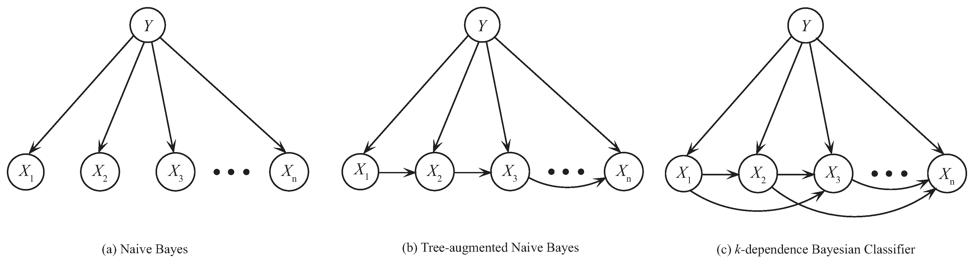
图中

• 箭头连接的两个节点: 这两个节点对应的随机变量直接相关.
• 无箭头链接的两个节点: 这两个节点对应的随机变量条件独立

Koller and Friedman (2009)

由于这样的独立性假设过强. 因此, 也发展出一些不那么 Naive 的版本 (e.g. 上图中的 b 和 c), 暂不在此展开.

3.2.2 拟合

包含交叉验证

# Import Multinomial Naive Bayes model
from sklearn.naive_bayes import MultinomialNB

# fit with multinomial naive bayes
model = MultinomialNB()
cv = cross_validate(model,
                    X=train_vector, 
                    y=train['label'], cv=5,
                    scoring='f1') # we can also set scoring='accuracy'
cv_scores = cv['test_score']
mean_cv = cv_scores.mean()
print('Fit time: {}'.format(cv['fit_time']))

Fit time: [0.00446224 0.00370574 0.00386596 0.00373578 0.00363111]

print('Score time: {}'.format(cv['score_time']))

Score time: [0.00291371 0.00208735 0.00212002 0.00211191 0.00200081]

print('CV scores: {}'.format(cv_scores))

CV scores: [0.8509434  0.86486486 0.85418627 0.87052342 0.87037037]

print('Mean of CV scores: {}'.format(round(mean_cv, 2)))

Mean of CV scores: 0.86

3.2.3 预测

# set model
model = MultinomialNB()

# Fit to data
model.fit(train_vector, train['label'])

MultinomialNB()

In a Jupyter environment, please rerun this cell to show the HTML representation or trust the notebook.
On GitHub, the HTML representation is unable to render, please try loading this page with nbviewer.org.

# Predict
test['label'] = model.predict(test_vector)
test['Keywords'] = test['title'].fillna('')
test[['uuid','Keywords','label']].to_csv('submit_task1_MultinomialNB.csv', index=None)

MultinomialNB 在 测试集 上的评分

将朴素贝叶斯的结果 (submit_task1_MultinomialNB.csv) 提交到竞赛平台 (外部链接). 得到的 F1_score 是 0.82315

这优于 Baseline 中使用的 LogisticRegression(), 后者得分为 0.67116

3.3 Benchmarking classifiers

本节根据 下面链接中给出的代码修改

https://scikit-learn.org/stable/auto_examples/text/plot_document_classification_20newsgroups.html#benchmarking-classifiers

Scikit-learn provides many different kinds of classification algorithms. In this section we will train a selection of those classifiers on the same text classification problem and measure both their generalization performance (accuracy on the test set) and their computation performance (speed), both at training time and testing time. For such purpose we define the following benchmarking utilities:

from sklearn import metrics
from sklearn.utils.extmath import density


def benchmark(clf, custom_name=False):
    print("_" * 80)
    print("Training: ")
    print(clf)
    cv = cross_validate(clf,
                    X=train_vector, 
                    y=train['label'], cv=5,
                    scoring='f1') # we can also set scoring='accuracy'
    cv_scores = cv['test_score']
    mean_cv_scores = cv_scores.mean()
    fit_time = cv['fit_time'].mean()
    score_time = cv['score_time'].mean()
    print('Mean Fit time: {}'.format(fit_time))
    print('Mean Score time: {}'.format(score_time))
    # print('CV scores: {}'.format(cv_scores))
    print('Mean CV scores: {}'.format(round(mean_cv_scores, 3)))

    if hasattr(clf, "coef_"):
        print(f"dimensionality: {clf.coef_.shape[1]}")
        print(f"density: {density(clf.coef_)}")
        print()

    print()
    if custom_name:
        clf_descr = str(custom_name)
    else:
        clf_descr = clf.__class__.__name__
    return clf_descr, mean_cv_scores, fit_time, score_time

from sklearn.ensemble import RandomForestClassifier
from sklearn.linear_model import LogisticRegression, SGDClassifier
from sklearn.naive_bayes import ComplementNB
from sklearn.linear_model import RidgeClassifier
from sklearn.neighbors import KNeighborsClassifier, NearestCentroid
from sklearn.svm import LinearSVC

results = []
for clf, name in (
    (LogisticRegression(), "Logistic Regression"),
    (RidgeClassifier(), "Ridge Classifier"),
    (KNeighborsClassifier(n_neighbors=10), "kNN"),
    (RandomForestClassifier(), "Random Forest"),
    # L2 penalty Linear SVC
    (LinearSVC(C=0.1, dual=False, max_iter=1000), "Linear SVC"),
    # L2 penalty Linear SGD
    (
        SGDClassifier(
            loss="log_loss", alpha=1e-4, n_iter_no_change=3, early_stopping=True
        ),
        "log-loss SGD",
    ),
    # NearestCentroid (aka Rocchio classifier)
    (NearestCentroid(), "NearestCentroid"),
    # Sparse naive Bayes classifier
    (ComplementNB(), "Complement naive Bayes"),
    # Multinomial naive Bayes classifier
    (MultinomialNB(), "Multinomial naive Bayes"),
):
    print("=" * 80)
    print(name)
    results.append(benchmark(clf, name))

================================================================================
Logistic Regression
________________________________________________________________________________
Training: 
LogisticRegression()
Mean Fit time: 0.7315375804901123
Mean Score time: 0.0014632701873779296
Mean CV scores: 0.982

================================================================================
Ridge Classifier
________________________________________________________________________________
Training: 
RidgeClassifier()
Mean Fit time: 0.23716230392456056
Mean Score time: 0.0013489723205566406
Mean CV scores: 0.942

================================================================================
kNN
________________________________________________________________________________
Training: 
KNeighborsClassifier(n_neighbors=10)
Mean Fit time: 0.0018662452697753907
Mean Score time: 0.2689769744873047
Mean CV scores: 0.123

================================================================================
Random Forest
________________________________________________________________________________
Training: 
RandomForestClassifier()
Mean Fit time: 4.879326820373535
Mean Score time: 0.039105796813964845
Mean CV scores: 0.925

================================================================================
Linear SVC
________________________________________________________________________________
Training: 
LinearSVC(C=0.1, dual=False)
Mean Fit time: 0.5811955451965332
Mean Score time: 0.0012734413146972656
Mean CV scores: 0.983

================================================================================
log-loss SGD
________________________________________________________________________________
Training: 
SGDClassifier(early_stopping=True, loss='log_loss', n_iter_no_change=3)
Mean Fit time: 0.01621556282043457
Mean Score time: 0.0010998249053955078
Mean CV scores: 0.979

================================================================================
NearestCentroid
________________________________________________________________________________
Training: 
NearestCentroid()
Mean Fit time: 0.005644369125366211
Mean Score time: 0.022679662704467772
Mean CV scores: 0.79

================================================================================
Complement naive Bayes
________________________________________________________________________________
Training: 
ComplementNB()
Mean Fit time: 0.0037185192108154298
Mean Score time: 0.0020303249359130858
Mean CV scores: 0.862

================================================================================
Multinomial naive Bayes
________________________________________________________________________________
Training: 
MultinomialNB()
Mean Fit time: 0.003662586212158203
Mean Score time: 0.0020671844482421874
Mean CV scores: 0.862


/Users/wgao/miniforge3/envs/datawhale-nlp/lib/python3.11/site-packages/threadpoolctl.py:1019: RuntimeWarning: libc not found. The ctypes module in Python 3.11 is maybe too old for this OS.
  warnings.warn(

3.4 结果与讨论

3.4.1 实验结果

• 朴素贝叶斯 在交叉验证中的平均得分是 0.862, 而测试集上的得分是 0.82315
• 逻辑回归 在交叉验证中的平均得分是 0.982, 而测试集上的得分是 0.67116

竞赛平台每日有三次提交机会. 其他模型的预测结果尚未提交

3.4.2 讨论

交叉验证会低估误差 (geekoverdose 2016). 然而, 即便如此, 上一节 (实验结果) 中的交叉验证中的得分也过于乐观了. 因此, 有理由考虑其他招致导致这种差异的因素.

比如, 考虑到 验证集 (Validation set) 与测试集 (Test set) 存在以下一点显著不同:

• 验证集由训练集划分而来. 它们包含原始论文的 Keywards,
• 测试集并不包含原始论文的 Keywards.

我猜测 (未验证), 论文的 Keywards 比 Abstract 更高浓度地指示着论文的分类. 因此, 可能导致过拟合.

3.5 总结

本节中

1. 我用 Baseline (Chapter 2) 中的代码导入数据 + 文本数据的向量化.
2. 我先尝试了 朴素贝叶斯 (MultinomialNB)
3. 接着, 我对比常见机器学习模型在本数据上的效果
4. 最后, 我尝试分析为什么 (在训练集上进行) 交叉验证拿到的得分 与 (在测试集的预测) 在竞赛平台上的得分相去甚远.

3.5.1 展望

• 如果希望进一步研究每个机器学习中涉猎的分类器. 那么有必要自己手写一个交叉验证函数
• 否则, 可以看看各种深度学习方法.

geekoverdose. 2016. “Answer to "Cross-Validation Misuse (Reporting Performance for the Best Hyperparameter Value)".” https://stats.stackexchange.com/a/224290.

Jordan, Michael I. 2004. “Graphical Models.” Statistical Science 19 (1): 140–55. https://doi.org/10.1214/088342304000000026.

Koller, Daphne, and Nir Friedman. 2009. Probabilistic Graphical Models: Principles and Techniques. MIT Press.